Deep-Sea AUV Navigation Using Side-scan Sonar Images and SLAM
요약
SSS를 활용한 underwater SLAM 관련 리뷰논문이다.
2010년도 OCEANS 학회논문이지만 사실상 다루는 내용이 전반적인 자료 조사와 내용 요약이어서, 실질적으로 리뷰논문처럼 읽었다. Citation은 14 회로, 적다.
Underwater SLAM에 활용되는 다양한 센서와 그 특징을 다루고, SSS의 특징과 그를 활용한 3D geometry reconstruction의 다양한 방법에 관해 다룬다.
이후 그 data를 활용한 underwater SLAM 논문 사례를 소개하고, 저자의 SLAM 프로젝트를 간략하게 소개하며 논문을 마친다. 본 포스트에서는 해당 프로젝트는 다루지 않았다.
내용 정리
I. Introduction
-
본 논문은 작성 시점 기준(2010) sonar data를 사용한 underwater SLAM 의 다양한 approaches를 다룬다.
-
“Underwater SLAM” 의 주된 장벽은 아래와 같다.
- SLAM 은 known features와 명확하게 관련되며, 반복적으로 관찰되는 feature에 크게 의존한다(landmark).
- Underwater 에서 optical camera는 유의미한 정보를 제공하기 어렵다.
II. Sensors for Underwater Navigation and Localization
A. Dead Reckoning
- 시작 위치에서 위치의 변화량을 누적시켜 현재 위치를 추정하는 방법이다.
- 사용하는 센서는 Accelerometer, 자이로스코프, 자력계, depth sensor 등이 있다.
- 센서의 오차와 수중에서의 지속적인 disturbances로 인해 몇 분 이상의 운용에서는 그 정확도를 장담할 수 없다.
B. Long Baseline (LBL)
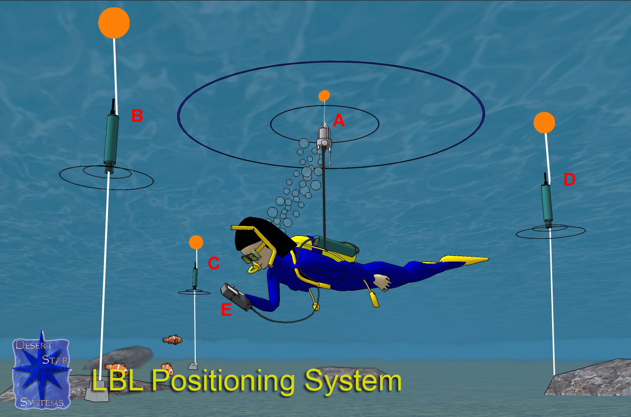
Fig.1 Long baseline
-
해저면의 known location에 acoustic transducer를 다수 설치하여 trilateration 을 기반으로 목표의 위치를 추정한다.
-
높은 정확도를 가지나, mission area가 설치된 transducers와 멀리 떨어질 경우 그 정확도가 떨어진다.
C. GNSS Aided Ultrashort Baseline
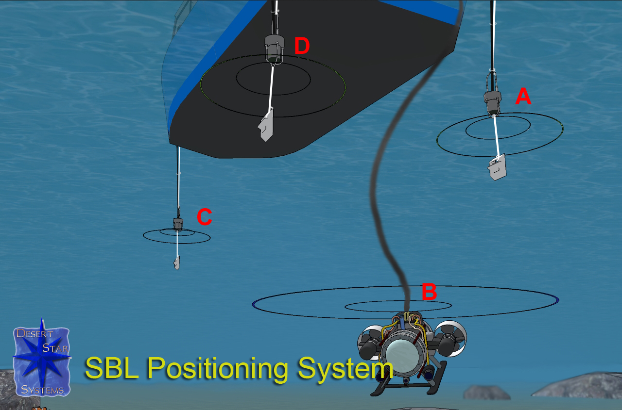
Fig.2 Short baseline
GNSS는 Global Navigation Satellite System으로, 위성항법시스템으로 주로 번역된다. ultrashort baseline(USBL)은 수상함에서 acoustic signal을 AUV에 전송하여 answer beacon의 신호를 바탕으로 AUV의 위치를 추정한다. LBL과 마찬가지로, 정확도가 높으나 mission area가 수상함과의 교신 가능 범위를 크게 벗어나지 못한다는 단점이 있다.
D. Cameras - Gated Viewing
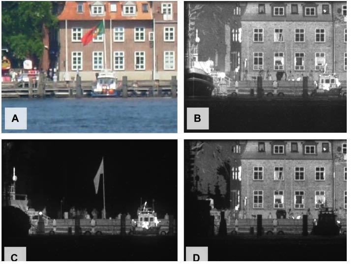
Fig.3 Gated viewing
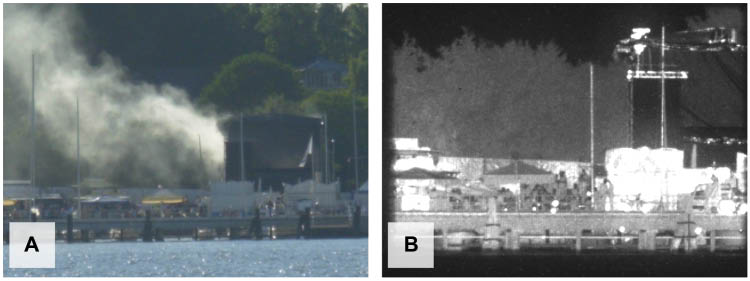
Fig.4 Gated viewing
수중에서 광학 데이터를 쓰기 어려운 이유는 아래와 같다:
-
전자기파의 높은 감쇄율로 인해 짧아진 가시거리(~60 m at best)
-
빛을 비춰도 수중의 입자들이 빛을 반사하기 때문에, 눈이 많이 오는 날 하이빔을 쏠 때의 모습과 비슷한 데이터가 생긴다.
-
이러한 한계를 극복하기 위해 gated viewing 이라는 방법을 사용한다.
- 이는 셔터 시간을 매우 짧게 조절하여 입자에 의해 scattered light의 양을 줄이고, 일정 거리 범위 내의 시야를 수신하는 방법이다.
- 이는 지상에서도 레이저 등을 활용해 안개나 연기 등에 의한 시야 차단을 극복하는데 쓰이기도 한다.
- 단, 매우 짧은 시간동안 셔터를 열 수 있는 카메라가 필요하며, 노출 시간이 매우 짧기 때문에 그만큼 광량이 많이 필요하단 점이 있다.
E. Sonar Sensors
광학 신호에 비해 감쇄가 훨씬 적은 점, 높은 지향성의 빔을 사용하면 그 해상도가 높아지는 점 등으로 소나 센서가 underwater에서의 the de facto standard로 활용되고 있다. 단점으로는, wave의 간섭으로 생기는 speckle noise, geometric distortion 등이 단점으로 알려져 있다.
본 논문에서는 side-scan sonar(SSS)와 multi-beam sonar를 다룬다.
1) Side-scan Sonars

Fig.5 Side-scan sonar
-
Towfish의 진행 방향으로는 매우 높은 지향성, 수직 방향으로는 넓은 빔폭을 가지고 있는 음향 신호를 사용한다.
-
해저 지형 reconstruction은 ill-posed inverse problem이다.
-
주로 사용되는 가정은 isovelocity, 그리고 scattered light에 대해선 Lambertian surface이다.
해저 지형 관련해 Shape-from-Shade(SfS) 라는 기법도 있다, 이는 Section IV에서 자세히 다뤄질 예정.
2) Multi-beam Sonar
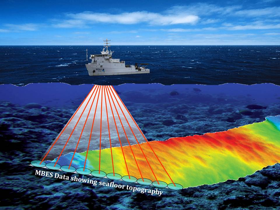
Fig.6 Multi-beam sonar
-
LiDAR과 유사함
- SSS가 현측에 transducer가 하나씩, 진행 방향으로만 narrow한 beam을 방사하는 것과는 달리, multi-beam sonar는 multiple transducer를 활용해 다수의 narrow beam을 사용한다(medical ultrasonic transducer와 유사한 것으로 보임)
- 때문에 3D information을 바로 얻을 수 있다.
- SSS보다 비교적 resolution이 낮아서, 정확한 shape가 필요한 task보단 sediment classification 같은 task에 적합하다.
III. Ambiguity of Side-scan Sonar Returns
-
SSS data로부터의 3D reconstruction은 ill-posed inverse problem
-
같은 지형이어도 측정한 위치와 각도에 따라 데이터가 크게 달라짐
A. Challenges in Extracting Elevation Problems
여기선 SSS 데이터를 사용하여 해저 지형의 높이를 추정할 때의 어려운 점을 소개한다.
- Acoustic signal에 영향을 주는 요소들:
- 입사각
- 거리
- 지형의 재질(의 acoustic impedance)
- Surface, volume scattering
- Absorption, dispersion properties
- 음속
- 해류
- Multipath propagation(e.g., 해수면, 해저면 반사 등)
- 빔패턴
- 주로 사용되는 가정들:
- Lambertian surface scattering
- No volume scattering
- Isovelocity
- Flat seabed
- Surface smoothness(=continuous, differentiable)
- Absorption, 해류 무시
- Multipath propagation 무시(time-gated pulse 사용으로 delayed signal 무시)
- 빔패턴은 이미 sonar spec. 으로 알고있거나, 실시간으로 estimation 가능 (원본 논문 fig 4-7 다시 그려서 올리기)
- Shadowed area의 정보가 없음
- Foreshortening
- 소나 이미지는 polar coordinate에서 $\theta$ 정보가 없다는 특성 상, 경사진 지형의 길이 데이터가 실제보다 훨씬 짧게 보이는 현상이 생긴다.
- Change of side-scan resolution
- Along-track
- SSS의 진행 방향에 대해서, beam width로 인해 지형의 거리가 멀 수록 resolution이 떨어질 수 밖에 없다.
- Varying vessel spd. 에 의해서도 sonar image에 왜곡이 생길 수 있다. * Across-track
- Polar coordinate 특성 상, 거리에 따라 해저면 구조물의 resolution이 달라질 수 있다.
즉, SSS는 비용이 낮으며 data가 easily visualized 되지만 그 해석과 3D reconstruction은 까다롭다는 특징이 있다.
B. Simulators for Side-scan Imagery
- 이미 1997년에 ray-tracing based simulator 논문이 있음[2]
- Velocity gradient
- Absorption loss
- Spreading loss 등의 익숙한 음향학 요소가 적용되어 있고, triangular facet에 대해 intersecting line 으로 계산하는 논문이다.
- SSS data로부터 3D reconstruction은 ill-posed inverse problem이라면, simulation은 forward problem이라고 할 수 있다.
IV. Elevation Information from Side-scan Data
- SLAM 에 활용하기 위한 3D data reconstruction
A. Estimating Elevation from Shadows
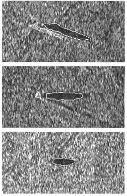
Fig.7 Co-operative statistical snake
- Co-operative Statistical Snake(CSS)[3]
- Shadowed region과 object(highlighted)를 detection
- Markov Random Field(MRF)를 사용해 shadow region을 분리
- Mode filter를 iteration해 shadow region의 intensity를 통일
- CSS는 object-highlight 와 shadow를 segmentation
- Highlighted, shadowed, background region의 grey-level을 기반으로 probability density function(pdf)
- Maximum likelihood estimation 을 기반으로 window function을 작성하여 highlighted region, shadowed region을 둘러싸는 snake를 찾는다.
그런데 statistical snake에 관해 구글링해도 잘 나오지 않는 게, 이미 시간이 꽤 지나 deep learning을 이용한 segmentation이 대세가 되어서 그런 게 아닐까 싶다.
B. Propagation Shape-from-Shading
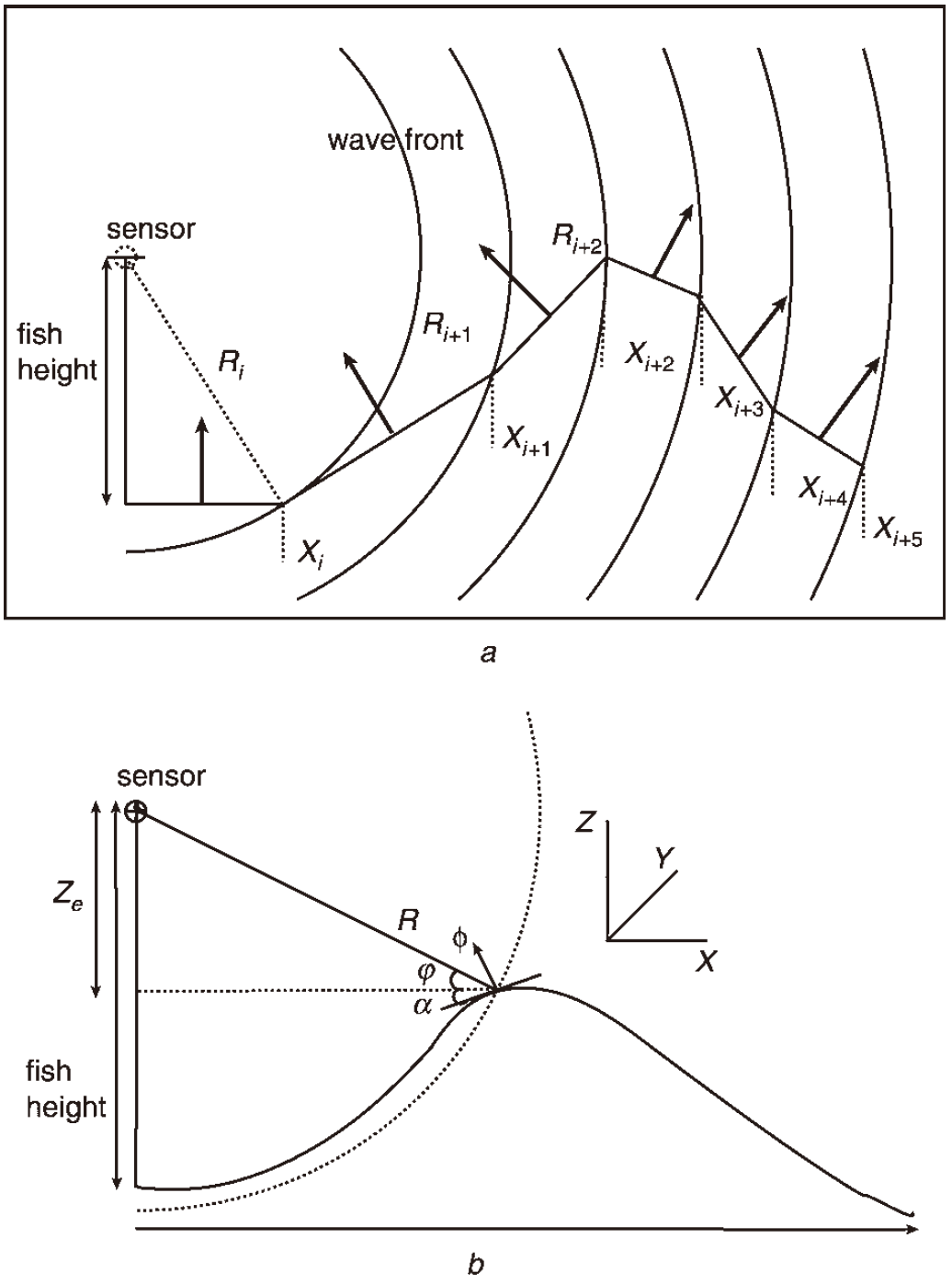
Fig.8 Shape from shadows
- SSS data의 line by line으로 3D reconstruction을 수행하는 방법 중 하나[4]
- The towfish의 바로 아래의 해저면(SSS data centerline으로부터의 first greatest difference of grey-level value)은 towfish에 대해 normal한 면으로 가정
- Lambertian scattering model을 기반으로 SSS data에서 지형에 반사된 각도를 계산
- 각 data point의 각도를 기반으로 seabed의 inclination angle을 계산하여 해저 지형을 3D reconstruction
- 2D median filter, graduated non-convexity filter 로 noise는 지우면서 outlier robustness를 확보
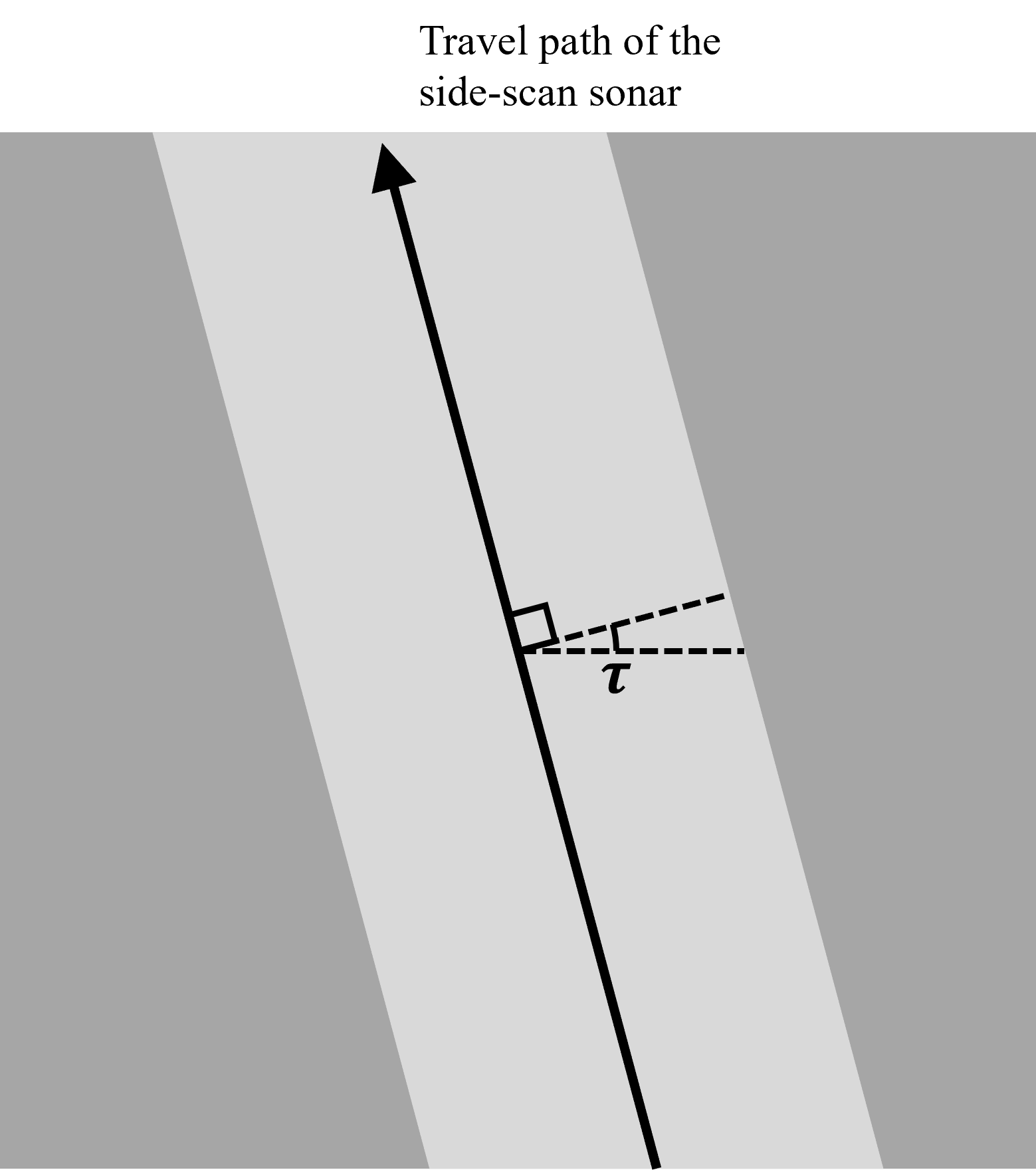
Fig.9 Path of the side-scan sonar and tilt angle $\tau$
- 왜 sonar image에 Fourier transform($F(\omega, \theta)$)을 하는가?
- 소나 이미지를 Fourier transform 한 수식은 아래와 같다.[5]
\begin{equation*} F(\omega, \theta) = I_i \mu i [\omega F_H ( \omega, \theta ) ] [\cos(\theta + \tau)] [\sin 2\sigma] \end{equation*}
여기서 $I_i$ 는 incident intensity, $\mu$는 empirically defined reflectivity coefficient, which is dependent on the sediment type, i 는 허수, $\theta$는 x축에 대한 각도, $\tau$는 위 그림에서 확인할 수 있는 tilt angle이다.
- (a) 소나 이미지의 freq. domain representation 은 slant angle($\sigma$)와 관련되어 있다 $F(\omega, \theta) \propto \cos(2\sigma) $
- (b) 소나 이미지는 seabed height map의 directional filtered 된 것이고, 이 directional filter는 tilt angle($\tau$)에 대한 코사인 함수와 연관되어 있다(i.e., $ F(\omega, \theta) \propto \cos(\theta + \tau) $)
C. Linear Shape-from-Shading
- 앞서 propagation shape-from-shading 과정에서 Fourier transformed intensity가 nonlinear eqn. 인데, 이를 linear eqn. 으로 근사[6]
- Nonlinear components를 Wiener filter로 제거
- 노이즈 $N(\omega, \theta)$ 는 $\sin(2\sigma) \cos(\theta+\tau)$ 에 비례한다고 가정
- 표면을 fractal Brownian function으로 가정하여 power spectrum이 $w^{-4}$ 에 비례
$\therefore$ Propagation SfS는 processing ripples에 robust하고,
linear SfS는 noise와 processing isotropic seabed 에 robust하다.
D. Hierarchical Recovering of Shape from Side-scan Data
- Expectation-maximization approach with gradient descent 방법을 사용하여, wave intensity의 모델 eqn.을 기반으로 해저면의 형상의 최적해를 구한 논문이 있다. [7]
- Lambertian scattering 을 기반으로, normalization constant, intensity of illuminating sound wave, reflectivity of the seafloor, 그리고 incidence angle 으로 returning wave의 intensity를 계산한다.
- 여기서 incidence angle은 ray의 벡터와 해저면의 벡터를 기반으로 작성할 수 있으므로, the model eqn. of wave intensity를 initial intensity, reflectivity, 그리고 ray 와 해저면의 벡터로 작성할 수 있다.
- The model eqn. of wave intensity를 기반으로, 실제 sonar image data와 비교하여 least mean-square error 기법으로 해저 지형의 최적해를 찾아낸다.
V. SLAM on Sonar Data
-
SLAM: Motion model과 반복적으로 관찰되는 특징점 데이터(landmark)를 활용해 vehicle의 localization 및 mapping의 uncertainties의 범위를 줄이는 기법
-
The process가 robust하려면 landmark가 잘 인식되고, 다른 특징점과 명확히 구분되어야 한다.
-
앞서 section III에서 소개한 SSS data의 한계로 인해, raw data로는 다른 위치와 각도에서 같은 landmark 인식이 어렵다.
-
때문에 section IV의 3D reconstruction이 동반되어야 한다.
A. SLAM on Side-scan Data
- SSS와 forward-looking sonar를 이용해 Extended Kalman filter SLAM(EKF-SLAM)을 수행한 논문이 있다. [8]
- 칼만 필터의 output을 smoothing하기 위해 Rauch-Tung-Striebel(RTS) backward filter가 사용되었다.
- Optimal smoothing
- $0 \leq t \leq T $ 인 real-time data가 있을 때,
Estimation 은 $0-t$ 까지의 data만 사용하지만,
Smoothing은 $0-T$ 의 data를 사용한다. - Optimal smoother는 two optimal filter, forward filter와 backward filter로 구성되어 있다.
- Forward filter는 t 이전의 모든 data를 사용하여 estimate $ \hat{x}_f $
- Backward filter는 t 이후의 모든 data를 사용하여 estimate $ \hat{x}_b $
- $0 \leq t \leq T $ 인 real-time data가 있을 때,
\begin{equation*} \hat{x} = A \hat{x}_f + B \hat{x}_b \end{equation*}
\begin{equation*} \begin{cases} \displaylines { \hat{x} = \textbf{P} ( \textbf{P}_f ^{-1} \hat{x}_f + \textbf{P}_b ^{-1} \hat{x}_b ) \\ \textbf{P}^{-1} = \textbf{P}_f ^{-1} + \textbf{P}_b ^{-1} } \end{cases} \end{equation*}
-
여기서 $\textbf{P}, \textbf{P}_f, \textbf{P}_b$ 는 각각
error covariance of smoothed estimate,
error covariance of forward estimate,
error covariance of backward estimate 이다. -
At the time $t=T$에서는 $ \textbf{P} = \textbf{P}_f $ 이고,$ \textbf{P}_b : \textbf{P}_b^{-1} = 0 $ 이다.
-
이 방법으로 forward Kalman filter를 먼저 수행하고, 이후에 backward RTS eqn. 을 수행한다.
-
For linear systems,
\begin{equation*} \displaylines { \hat{x}(k|N) = \hat{x}_f (k \ \ k) + \textbf{A}(k)[ \hat{x}(k+1|N) - \hat{x}_f(k+1 \ \ k) ] \\ \textbf{A}(k) = \textbf{P}_f(k \ \ k) \textbf{F}’ \textbf{P}_f ( k+1 \ \ k )^{-1} \\ \textbf{P}(k|N) = \textbf{P}_f(k \ \ k) + \textbf{A}(k) \times [ \textbf{P}(k+1 \ \ N) - \textbf{P}_f(k+1|k) ] \textbf{A}(k)’ } \end{equation*}
- 여기서 $ \hat{x}_f(k | k) $ 와 $ \hat{x}_f(k+1 \ \ k) $는 prediction 및 correction state of the forward filter at instant k, $ \textbf{P}_f(k \ \ k) $와 $ \textbf{P}_f(k+1 \ \ k) $는 각각의 respective covariance이다.
$ \hat{x}(k \ \ N) $ 과 $ \textbf{P}(k \ \ N) $ 은 각각 time instant k에서 smoothed estimate 와 error covariance이다.
$\textbf{F} $ 는 transition matrix이다.
B. SLAM in Structured Environments
-
PhD dessertation
-
소나를 vertically mount 하여 회전시켜 촬영해 360도 이미지를 획득하였는데, 빔 패턴을 고려하면 forward looking sonar를 yaw 방향으로 회전시킨 것과 동일하다.
C. 3D SLAM on Sonar Data
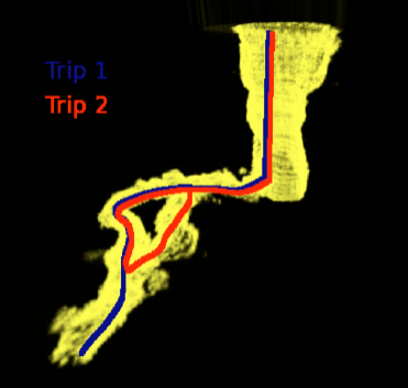
Fig.10 3D SLAM in an underwater tunnel
- Rao-Blackwellized Particle Filter(RBPFs) 기반 SLAM으로 underwater tunnel에서 3D SLAM을 수행[9]
-
또한, 해당 논문에서는 Deffered Reference Counting Octrees(DRCO) 라는 data structure를 제안하여, SLAM 과정에서의 메모리를 최적화하였다.
-
그 결과, 10k 의 SLAM iteration에서도 10 m 미만의 localization error를 기록하였다.
참고문헌
[1] P. Woock and C. Frey, “Deep-sea AUV navigation using side-scan sonar images and SLAM,” OCEANS’10 IEEE SYDNEY, 2010, pp. 1-8, doi: 10.1109/OCEANSSYD.2010.5603528.
[2] J. M. Bell and L. M. Linnett, “Simulation and analysis of synthetic sidescan sonar images,” IEE Proceedings -Radar, Sonar and Navigation, vol. 144, no. 4, pp. 219–226, Aug. 1997.
[3] S. Reed, Y. Petillot and J. Bell, “An automatic approach to the detection and extraction of mine features in sidescan sonar,” in IEEE Journal of Oceanic Engineering, vol. 28, no. 1, pp. 90-105, Jan. 2003, doi: 10.1109/JOE.2002.808199.
[4] D. Langer and M. Hebert, “Building qualitative elevation maps from side scan sonar data for autonomous underwater navigation,” Proceedings. 1991 IEEE International Conference on Robotics and Automation, 1991, pp. 2478-2483 vol.3, doi: 10.1109/ROBOT.1991.131997.
[5] Bell, J. M., Chantler, M. J., & Wittig, T. (1999). Sidescan sonar: a directional filter of seabed texture? IEE Proceedings - Radar, Sonar and Navigation, 146(1), 65. doi:10.1049/ip-rsn:19990266
[6] E. Dura, J. M. Bell, and D. M. Lane, “Reconstruction of textured seafloors from side-scan sonar images,” IEE Proceedings – Radar, Sonar and Navigation, vol. 151, no. 2, pp. 114–126, Apr. 2004.
[7] E. Coiras, Y. Petillot and D. M. Lane, “Multiresolution 3-D Reconstruction From Side-Scan Sonar Images,” in IEEE Transactions on Image Processing, vol. 16, no. 2, pp. 382-390, Feb. 2007, doi: 10.1109/TIP.2006.888337.
[8] I. Tena Ruiz, S. de Raucourt, Y. Petillot and D. M. Lane, “Concurrent mapping and localization using sidescan sonar,” in IEEE Journal of Oceanic Engineering, vol. 29, no. 2, pp. 442-456, April 2004, doi: 10.1109/JOE.2004.829790.
[9] N. Fairfield, G. A. Kantor, and D. Wettergreen, “Real-Time SLAM with Octree Evidence Grids for Exploration in Underwater Tunnels,” Journal of Field Robotics, vol. 24, no. 1-2, pp. 03–21, 2007.
Leave a comment